Authors:
(1) J. Quetzalcóatl Toledo-Marín, University of British Columbia, BC Children’s Hospital Research Institute Vancouver BC, Canada (Email: [email protected]);
(2) James A. Glazier, Biocomplexity Institute and Department of Intelligent Systems Engineering, Indiana University, Bloomington, IN 47408, USA (Email: [email protected]);
(3) Geoffrey Fox, University of Virginia, Computer Science and Biocomplexity Institute, 994 Research Park Blvd, Charlottesville, Virginia, 22911, USA (Email: [email protected]).
Table of Links
2 Methods
The steady state of the diffusion equation is precisely the convolution of the equation’s associated Green’s function and the initial state. Hence a naive approach would consider a deep convolutional NN (CNN) where the height and width in each layer is kept fixed and equal to the input. CNNs are good at detecting edges and as the number of convolution layers increases, the CNN can detect more sophisticated elements. So can a CNN predict the stationary solution? We argue that it would require a large number of convolution layers such that each convolution would be proportional to a timestep. Adding many convolutions would lead to a rather harder and slower training, as it would increase the chances of under or overflow in the gradient. Furthermore, the number of convolution layers would need to be variable is some form or fashion in order to mimic the timesteps required to reach the stationary solution given an initial condition. There are ways to address each of the previous setbacks but there’s also a trade-off for every decision (e.g., increasing the number of convolutional layers increases the model’s instability which can be addressed by adding more regularization layers which makes the model larger and requires more time to train). Experience tells us that deep convolutional NNs where the height and width in each layer is kept fixed and equal to the input are not good for our task [17].
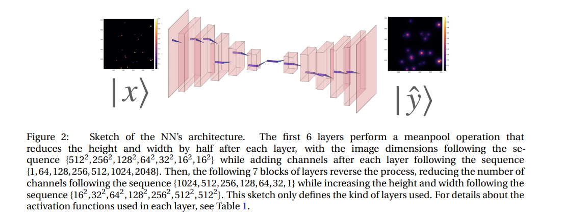
We designed and built an encoder-decoder CNN (ED-CNN) as our architecture. Fig. 2 provides a sketch of our NN architecture. We denote by |x〉 and |yˆ〉 the input and output images, that is the initial condition layout of the source cells and the predicted stationary solution of the diffusion equation, respectively. The input |x〉 goes through convolutional blocks depicted in Fig. 2 and generates the prediction |yˆ〉 which we then compare with the ground truth |y〉. The core feature of an encoder-decoder is the cone-like structure whereby the information is being compressed when it reaches the bottle neck and then it’s decompressed.
Consider the following: A CNN can be seen as a set of operators {Oi} acting on the input, i.e.,

where the i tags the convolutional layer. Notice that in the particular case where {Oi} are unitary linear operators and all the same O = 1− Ad t, Eq. (1) becomes

Notice that the previous Eq. is akin to a ResNet architecture [19]. By defining d t = t/n, where t is time, and taking the limit n → ∞ leads to |yˆ〉 = exp(At)|x〉. Hence, when |yˆ〉 equals the ground truth |y〉, the CNN has learnt the operator exp(At). Notice that taking the derivative with respect to time leads to the diffusion equation:

Typically, numerical methods for searching for the stationary solution of a diffusion equation operate by comparing the solution at time t with the solution at time t +∆t, and halting the process when the difference between |y(t)〉 and |y(t+∆t)〉is smaller in magnitude than some pre-determined error value. However, the time t at which the stationary solution is reached depends on the initial conditions and the inhomogeneity term in the diffusion equation. This analogy suggests that, similar to traditional numerical methods, CNNs also require a flexible number of layers to reach the stationary solution, rather than an infinite number of layers. There have been recent developments in addressing the issue of a variable number of layers. For example, in reference [20], the authors propose a method in which the dropout parameters are trained in conjunction with the model parameters.
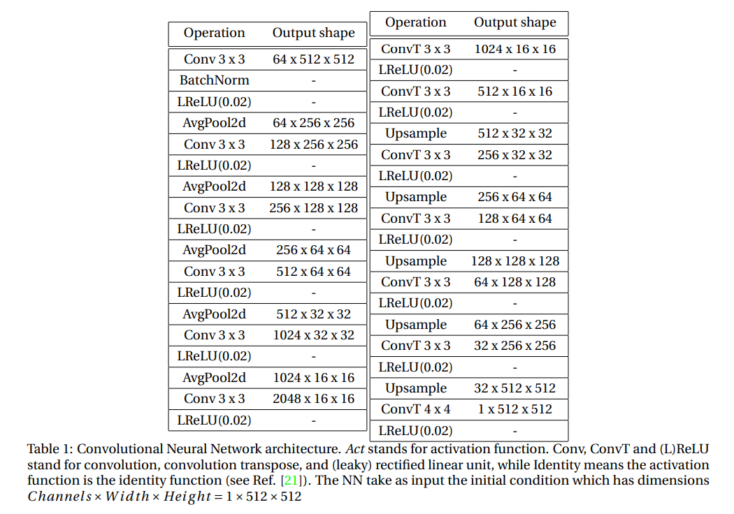
In the context of ED-CNNs, it is a widely held belief that the cone-like architecture leads to improved performance due to the compression in the bottleneck. However, we argue that this is not the sole, if any, contributing factor. It is important to note that the ED-CNN architecture involves summing over the lattice and introducing a new variable, the depth. Additionally, past the bottleneck, the ED-CNN projects back to the original space. In this sense, we say the ED-CNN learns a propagator in a reciprocal space similar to methods such as Laplace and Fourier transform. In Table 1 we specify the neural network by specifying the type of operation and output shape through the sequence of blocks in the NN. Notice that the bottleneck block is 2048∗16∗16 which is twice the size of the input.
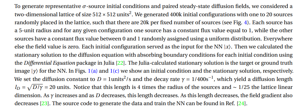
We built and trained the NN in PyTorch. We used ADAM as the optimizer [25]. Deciding on a loss function is a critical choice in the creation of the surrogate. The loss function determines the types of error the surrogate’s approximation will make compared to the direct calculation and the acceptability of these errors will depend on the specific application. The mean squared error (MSE) error is a standard choice. However, it is more sensitive to larger absolute errors and therefore tolerates large relative errors at pixels with small values. In most biological contexts we want to have a small absolute error for small values and a small relative error for large values. We explored the
NN’s performance when trained using a set of different loss functions with different hyperparameters. The set of different loss functions we used were MAE, MSE, Huber loss [26] and inverse Huber loss defined as:
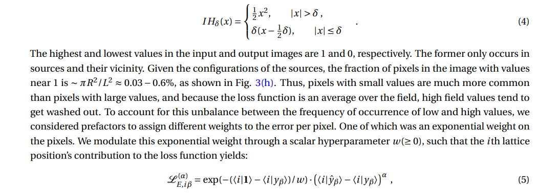
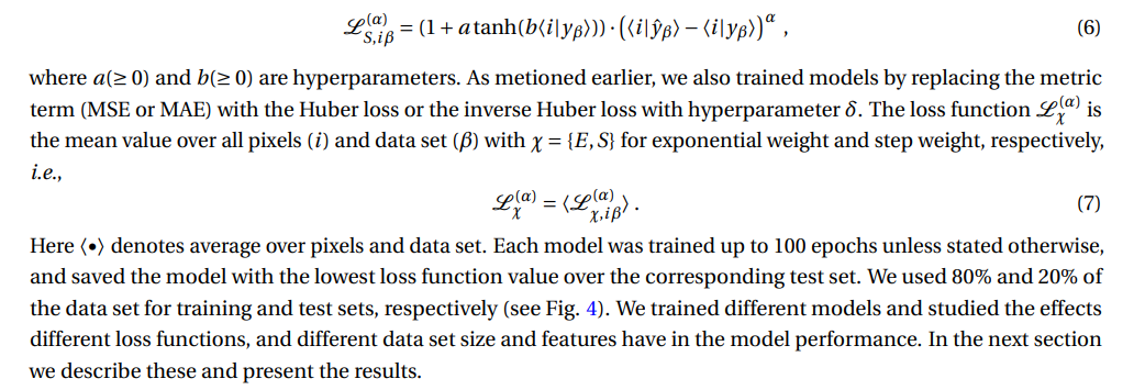
where α is 1 or 2 for MAE or MSE, respectively and β tags the tuple in the data set (input and target). Here 〈|〉 denotes the inner product and |i〉 is a unitary vector with the same size as |yβ〉 with all components equal to zero except the element in position i which is equal to one. |1〉 is a vector with all components equal to 1 and with size equal to that of |yβ〉. Then 〈i|yβ〉 is a scalar corresponding to the pixel value at the ith position in |yβ〉, whereas 〈i|1〉 = 1 for all i. Notice that high and low pixel values will have an exponential weight ≈ 1 and ≈ exp(−1/w), respectively. This implies that the error associated to high pixels will have a larger value than that for low pixels. Another prefactor we considered was a step-wise function, viz.
This paper is available on arxiv under CC 4.0 license.

